Capital Market Assumptions: Redefined
Capital markets assumptions are both commonplace and prone to inaccuracy. Rather than gaze into the crystal ball, in this paper we aim to help you improve on CMAs for yourselves.
Key takeaways:
- It is debateable whether the common 10-year timeframe represents an unconditional base rate, and using the same look-ahead for all assets may be an oversimplification
- Be prepared – returns to beta over the next decade are likely to be lower than we have seen over the last 10 years
- Approach capital market assumptions (CMAs) with healthy scepticism. Seek to understand their underlying drivers and assumptions before employing them in your strategic asset allocations
Introduction
CMAs seek to help allocators with their asset allocation decisions by establishing long-term forecasts for different financial assets. The problem is that they either fail to do this with much accuracy or make their forecasts with such a degree of caution that the output is of limited practical use.
In this paper, we propose a framework to help allocators to calculate these assumptions for themselves, as well as explore some practical applications for the resulting data.
A critical question that is not given sufficient consideration in our view is: what are you proposing to use CMAs for? There seem to be two options. First, allocators may have a liability window over the next 10 years, and want a base case for how assets might match these liabilities. Or secondly, they may want an unconditional base rate which serves as the foundation for ultra-long portfolio allocations. If the latter, and we suspect this is the case for most users, then the timeframe consideration becomes particularly important.
In Part One, we discuss forecast timeframes. In Part Two, we describe four credible methods for determining CMAs. In Part Three, we use findings from the prior two sections to calculate a range of CMAs for US stocks and 10-year Treasuries (UST10). These assumptions allow us, in Part Four, to derive strategic asset allocations (SAA), based on optimisation parameters such as return, volatility drawdown and Sharpe ratio.
In this paper we focus only on US equities and intermediate duration, as the two most consequential portfolio building blocks.
Part One: CMA timeframes
Inherent in CMAs is the idea that asset returns are more predictable on a long-term horizon than on a short-term view. In Figure 1, we show the distribution of one- and 10-year rolling returns to US stocks and bonds, over the ultra-long-term.
Figure 1. Distribution of returns for US stocks (top) and bonds (bottom), 1800-2024
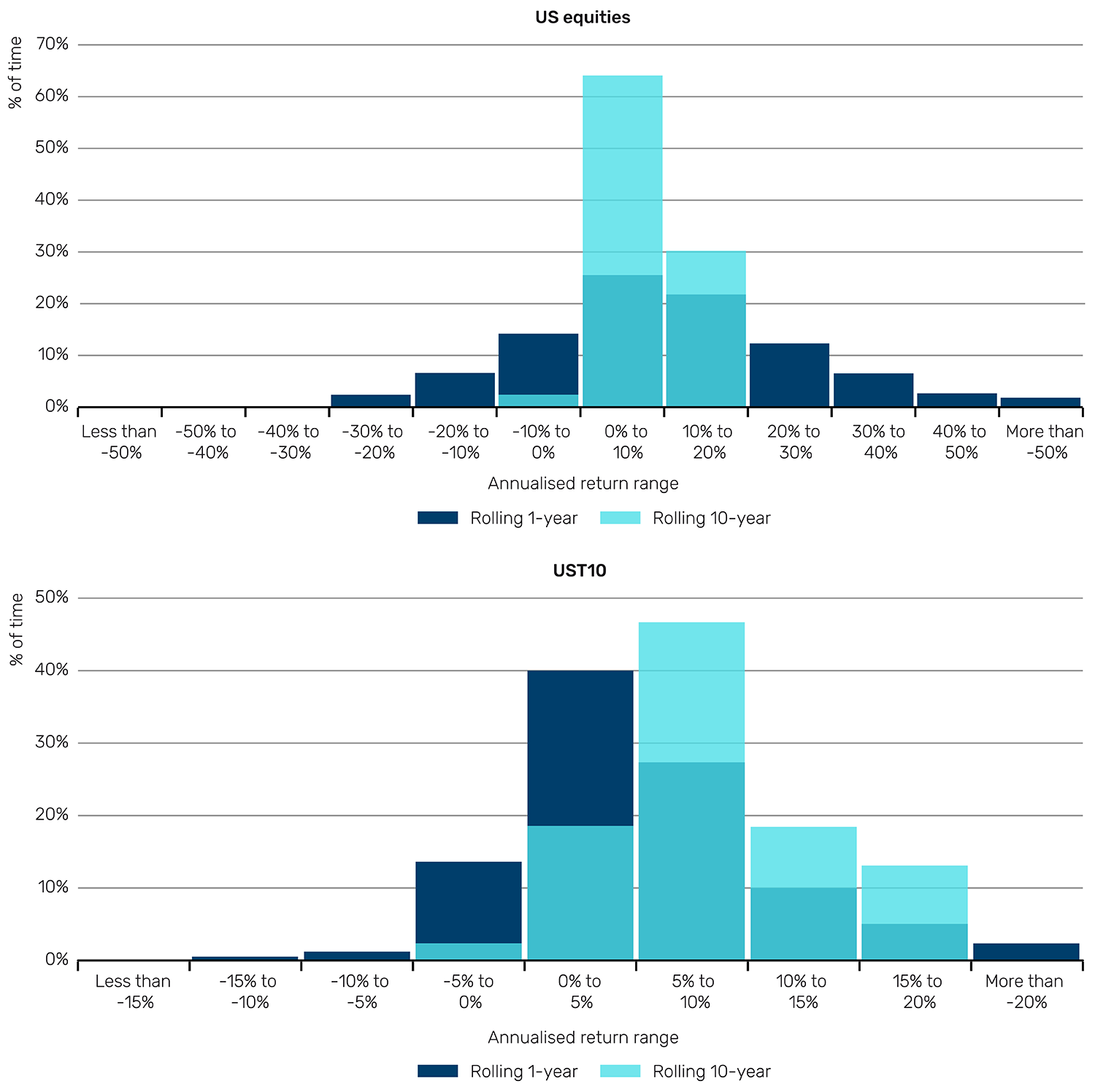
Source: GFD, Man Group. As of December 2024.
For stocks, the distribution becomes dramatically compressed as the return lookback is increased. On a 10-year annualised basis, 93% of returns fall into the 0-20% annual return buckets (on a one-year basis, the figure is 49%). However, the 10-year range is still wider than might be expected. There are 547 instances where returns were either below 4% annualised, or above 16% annualised, collectively accounting for over a fifth of history. Imagine that you’re a US$100 billion endowment or sovereign wealth fund advising your stakeholders on the kind of distributions they can expect based on long-term forecasts. These two pathways diverge by almost US$300 billion.
From Figure 1, we can also see that the distribution compresses more for equities than for bonds as the return window rises. For bonds, the 0-10% bands represent 68% of rolling one-year observations, and 66% of rolling 10-year periods.1
Most investors’ instinctive outlook duration is 10 years. But it is debatable whether this represents an unconditional base rate, at least considering historic precedent. In the case of equities, your forecast horizon might need to be longer than you think, and applying the same timeframe for all assets could risk oversimplification.
Part Two: CMA methodologies
With these limitations in mind, we now offer four credible methods for determining CMAs.
The simple historic method
The simple historic method looks at returns over the very long term, i.e., it is an aggregation of as much historic data as is attainable for the given asset. For US stocks, this has been 8.7% (1800 to 2024). For US bonds, this has been 5.0% over the same period.2
While this is a potentially attractive route to establishing an unconditional base rate, we would repeat the warning from Part One – the next 225 years could be very different to the last. To illustrate, consider that equities can be seen as a levered play on nominal GDP. The rate of nominal GDP growth in developed economies over long windows has been highly variable. In Figure 2, we show 225-year annualised nominal GDP growth for the UK for four discrete windows since 1270 (calculated from the Bank of England’s Millenium of Macroeconomic Data resource).
By all means, take an ultra-long history as a base rate to inform future expectations. But remember to hold it lightly.


Comments
Post a Comment